Rilostat

The ilostat R package in a few words

This R package provides tools to access, download and work with the data contained in ILOSTAT, the ILO Department of Statistics’ online database. ILOSTAT’s data and related metadata are also directly available through ILOSTAT’s website.

For more information on ILOSTAT’s R package, including contact details and source code, refer to its github page.

Introduction

The ILO’s main online database, ILOSTAT, maintained by the Department of Statistics, is the world’s largest repository of labour market statistics. It covers all countries and regions and a wide range of labour-related topics, including employment, unemployment, wages, working time and labour productivity, to name a few. It includes time series going back as far as 1938; annual, quarterly and monthly labour statistics; country-level, regional and global estimates; and even projections of the main labour market indicators.

ILOSTAT’s website provides immediate access to all its data and related metadata through different ways. Basic users can simply view the desired data online or download it in Excel or csv formats. More advanced users can take advantage of ILOSTAT’s well-structured bulk download facility (user guide), or the SDMX web service (user guide).

The ilostat R package ('Rilostat') was designed to give data users the ability to access the ILOSTAT database, search for data, rearrange the information as needed, download it in the desired format, and make various data visualizations, all in a programmatic and replicable manner, with the possibility of quickly re-running the queries as required.

Main features of the ilostat R package

Provides access to all annual, quarterly, and monthly data available via the ILOSTAT bulk download facility (user guide)
Allows to search for and download data and related metadata in English, French and Spanish
Gives the ability to return POSIXct dates for easy integration into plotting and time-series analysis techniques
Returns data in long format for direct integration with packages like ggplot2 and dplyr
Gives immediate access to the most recent updates
Allows for grep-style searching for data descriptions and names
Provides access to the ILOSTAT catalogue of related descriptive metadata (user guide)

Acknowledgements

The developer of this package drew extensive inspiration from the eurostat R package and its related documentation:

Retrieval and Analysis of Eurostat Open Data with the eurostat Package - Leo Lahti, Przemyslaw Biecek, Markus Kainu and Janne Huovari. R Journal 9(1), 385-392, 2017.

Installation

To install the release version, use the following command:

## Warning: package 'usethis' was built under R version 4.4.1

install.packages("Rilostat")

To install the development version, use the following command:

if(!require(devtools)){install.packages('devtools')}
install_github("ilostat/Rilostat")

The ilostat R package ('Rilostat') includes the following functions:

require(Rilostat)
as.data.frame(ls("package:Rilostat"))

##   ls("package:Rilostat")
## 1    clean_ilostat_cache
## 2           dataexplorer
## 3   distribution_ilostat
## 4            get_ilostat
## 5        get_ilostat_dic
## 6        get_ilostat_toc
## 7          label_ilostat

We do not expect to update the ilostat R package too often, but based on questions and remarks from ILOSTAT data users, we will progressively create more examples, tutorials, demos and apps. Please visite the Rilostat package website.

Search for data

Unless you already know the code of the indicator or the ref_area (reference area - countries or regions) that you want to download, the first step would be to search for the data you are interested in. get_ilostat_toc() provides grep style searching of all available indicators from ILOSTAT’s bulk download facility and returns the indicators matching your query. get_ilostat_toc(segment = 'ref_area') returns the datasets available by ref_area (‘country’ and ‘region’).

To access the table of contents of all available indicators in ILOSTAT (by indicator):

toc <- get_ilostat_toc()

Table 1a. Extract, ‘Table of contents by indicator in English’
id	indicator	indicator.label	freq	freq.label
SDG_0111_SEX_AGE_RT_A	SDG_0111_SEX_AGE_RT	SDG indicator 1.1.1 - Working poverty rate (percentage of employed living below US$2.15 PPP) (%)	A	Annual
SDG_0131_SEX_SOC_RT_A	SDG_0131_SEX_SOC_RT	SDG indicator 1.3.1 - Proportion of population covered by social protection floors/systems (%)	A	Annual
SDG_0552_NOC_RT_A	SDG_0552_NOC_RT	SDG indicator 5.5.2 - Proportion of women in senior and middle management positions (%)	A	Annual

All settings are available in the 3 official languages of the ILO: English ('en'), French ('fr') and Spanish ('es'). The default is 'en'.

For instance, to access the table of contents of all available datasets by reference area in ILOSTAT in Spanish:

toc <- get_ilostat_toc(segment = 'ref_area', lang = 'es')

Table 1b. Extract, ‘Table of contents by ref_area in Spanish’
id	ref_area	ref_area.label	freq	freq.label	data.start	data.end	last.update	n.records
AFG_A	AFG	Afganistán	A	Anual	1978	2026	01/09/2024 08:09:14	349914
AFG_Q	AFG	Afganistán	Q	Trimestral	2005Q1	2020Q1	24/03/2023 06:41:23	2163
AFG_M	AFG	Afganistán	M	Mensual	2005M01	2020M03	22/03/2023 22:03:17	6485

You can search for words or expressions within the table of contents listing all of ILOSTAT’s indicators.

For example, searching for the word “bargaining” will return the indicators containing that word somewhere in the indicator information:

toc <- get_ilostat_toc(search = 'bargaining')

Table 1c. ‘Table of contents by indicator with search word ’bargaining’’
id	indicator	indicator.label	freq	freq.label	data.start	data.end	last.update
SDG_0882_NOC_RT_A	SDG_0882_NOC_RT	SDG indicator 8.8.2 - Level of national compliance with labour rights (freedom of association and collective bargaining)	A	Annual	2015	2022	09/02/2024 09:48:27
ILR_CBCT_NOC_RT_A	ILR_CBCT_NOC_RT	Collective bargaining coverage rate (%)	A	Annual	2000	2020	03/05/2022 15:55:20

Similarly, you can also search the list of all available datasets by reference area for a given reference area (using a country or region name or code) or even for a given data frequency (annual, quarterly or monthly). The search also allows you to look for several alternative and/or additional items at once.

For instance, to look for datasets with annual data for either Albania or France:

toc <- get_ilostat_toc(segment = 'ref_area', search = c('France|Albania', 'Annual'), 
                                            fixed = FALSE)

Table 1d. ‘Table of contents by ref_area with search words ’France’ or ‘Albania’ and ‘Annual’’
id	ref_area	ref_area.label	freq	freq.label	data.start	data.end	last.update	n.records
ALB_A	ALB	Albania	A	Annual	1960	2030	01/09/2024 08:09:14	947892
FRA_A	FRA	France	A	Annual	1955	2030	01/09/2024 08:09:14	2313174

You can also manipulate ILOSTAT’s table of contents’ dataframe using the basic R filter. If you are already familiar with ILOSTAT data and the way it is structured, you can easily filter what you want.

For example, if you know beforehand you want data only from ILOSTAT’s Short Term Indicators dataset (code “STI”) and you are only interested in monthly data (code “M”) you can simply do:

toc <-  dplyr::filter(get_ilostat_toc(), collection == 'STI', freq == 'M')

Table 1e. Extract, ‘Table of contents by indicator filtered for Monthly Short term indicators’
id	indicator	indicator.label	freq	freq.label
POP_XWAP_SEX_AGE_NB_M	POP_XWAP_SEX_AGE_NB	Working-age population by sex and age (thousands)	M	Monthly
POP_XWAP_SEX_AGE_EDU_NB_M	POP_XWAP_SEX_AGE_EDU_NB	Working-age population by sex, age and education (thousands)	M	Monthly
POP_XWAP_SEX_AGE_GEO_NB_M	POP_XWAP_SEX_AGE_GEO_NB	Working-age population by sex, age and rural / urban areas (thousands)	M	Monthly
POP_XWAP_SEX_AGE_LMS_NB_M	POP_XWAP_SEX_AGE_LMS_NB	Working-age population by sex, age and labour market status (thousands)	M	Monthly
POP_XWAP_SEX_EDU_NB_M	POP_XWAP_SEX_EDU_NB	Working-age population by sex and education (thousands)	M	Monthly

Download data

The function get_ilostat() explores ILOSTAT’s datasets and returns datasets by indicator (default, segment indicator) or by reference area (segment ref_area). The id of each dataset is made up by the code of the segment chosen (indicator code or reference area code) and the code of the data frequency required (annual, quarterly or monthly), joined by an underscore.

Get a single dataset:

As stated above, you can easily access the single dataset of your choice through the get_ilostat() function, by indicating the code of the dataset desired (indicator_frequency or ref_area_frequency).

If you want to access annual data for indicator code UNE_2UNE_SEX_AGE_NB, you should type:

dat <- get_ilostat(id = 'UNE_2UNE_SEX_AGE_NB_A', segment = 'indicator')

## trying URL 'https://rplumber.ilo.org/data/indicator/?id=UNE_2UNE_SEX_AGE_NB_A&format=.rds'

## trying saving cache 'C:\Users\bescond\AppData\Local\Temp\Rtmpy4Fuzy/ilostat/indicator-UNE_2UNE_SEX_AGE_NB_A-code-raw-20240523T1439.rds'

Table 2a. Extract, ‘Annual unemployment by sex and age, ILO modelled estimates, Nov. 2018’
ref_area	source	indicator	sex	classif1	time	obs_value
AFG	XA:2198	UNE_2UNE_SEX_AGE_NB	SEX_T	AGE_YTHADULT_YGE15	2025	1351.730
AFG	XA:2198	UNE_2UNE_SEX_AGE_NB	SEX_T	AGE_YTHADULT_Y15-24	2025	591.161
AFG	XA:2198	UNE_2UNE_SEX_AGE_NB	SEX_T	AGE_YTHADULT_YGE25	2025	760.568

If you want to access all annual data available in ILOSTAT for Armenia:

dat <- get_ilostat(id = 'ARM_A', segment = 'ref_area')

## trying URL 'https://rplumber.ilo.org/data/ref_area/?id=ARM_A&format=.rds'

## trying saving cache 'C:\Users\bescond\AppData\Local\Temp\Rtmpy4Fuzy/ilostat/ref_area-ARM_A-code-raw-20240901T0809.rds'

Table 2b. Extract, ‘Armenia, annual data’
ref_area	source	indicator	sex	classif1	time	obs_value
ARM	XA:1931	SDG_0111_SEX_AGE_RT	SEX_T	AGE_YTHADULT_YGE15	2023	0.091
ARM	XA:1931	SDG_0111_SEX_AGE_RT	SEX_T	AGE_YTHADULT_YGE15	2022	0.092
ARM	XA:1931	SDG_0111_SEX_AGE_RT	SEX_T	AGE_YTHADULT_YGE15	2021	0.147

Get multiple datasets:

It is also possible to download multiple datasets at once, simply by setting the dataset’s id as a vector of ids or a tibble that lists ids in a specific column:

dat <- get_ilostat(id = c('AFG_A', 'TTO_A'), segment = 'ref_area')

## trying URL 'https://rplumber.ilo.org/data/ref_area/?id=AFG_A&format=.rds'

## trying saving cache 'C:\Users\bescond\AppData\Local\Temp\Rtmpy4Fuzy/ilostat/ref_area-AFG_A-code-raw-20240901T0809.rds'

## trying URL 'https://rplumber.ilo.org/data/ref_area/?id=TTO_A&format=.rds'

## trying saving cache 'C:\Users\bescond\AppData\Local\Temp\Rtmpy4Fuzy/ilostat/ref_area-TTO_A-code-raw-20240901T0809.rds'

dplyr::count(dat, ref_area)

## # A tibble: 2 × 2
##   ref_area      n
##   <chr>     <int>
## 1 AFG      349914
## 2 TTO      331294

toc <- get_ilostat_toc(search = 'CPI_')

dat <- get_ilostat(id = toc, segment = 'indicator', quiet = TRUE)

## trying URL 'https://rplumber.ilo.org/data/indicator/?id=CPI_XCPI_COI_RT_A&format=.rds'

## trying saving cache 'C:\Users\bescond\AppData\Local\Temp\Rtmpy4Fuzy/ilostat/indicator-CPI_XCPI_COI_RT_A-code-raw-20240718T0733.rds'

## trying URL 'https://rplumber.ilo.org/data/indicator/?id=CPI_XCPI_COI_RT_Q&format=.rds'

## trying saving cache 'C:\Users\bescond\AppData\Local\Temp\Rtmpy4Fuzy/ilostat/indicator-CPI_XCPI_COI_RT_Q-code-raw-20240718T0738.rds'

## trying URL 'https://rplumber.ilo.org/data/indicator/?id=CPI_XCPI_COI_RT_M&format=.rds'

## trying saving cache 'C:\Users\bescond\AppData\Local\Temp\Rtmpy4Fuzy/ilostat/indicator-CPI_XCPI_COI_RT_M-code-raw-20240718T0702.rds'

## trying URL 'https://rplumber.ilo.org/data/indicator/?id=CPI_NCPD_COI_RT_Q&format=.rds'

## trying saving cache 'C:\Users\bescond\AppData\Local\Temp\Rtmpy4Fuzy/ilostat/indicator-CPI_NCPD_COI_RT_Q-code-raw-20240718T0738.rds'

## trying URL 'https://rplumber.ilo.org/data/indicator/?id=CPI_NCPD_COI_RT_M&format=.rds'

## trying saving cache 'C:\Users\bescond\AppData\Local\Temp\Rtmpy4Fuzy/ilostat/indicator-CPI_NCPD_COI_RT_M-code-raw-20240718T0742.rds'

## trying URL 'https://rplumber.ilo.org/data/indicator/?id=CPI_NCYR_COI_RT_A&format=.rds'

## trying saving cache 'C:\Users\bescond\AppData\Local\Temp\Rtmpy4Fuzy/ilostat/indicator-CPI_NCYR_COI_RT_A-code-raw-20240718T0740.rds'

## trying URL 'https://rplumber.ilo.org/data/indicator/?id=CPI_NCYR_COI_RT_Q&format=.rds'

## trying saving cache 'C:\Users\bescond\AppData\Local\Temp\Rtmpy4Fuzy/ilostat/indicator-CPI_NCYR_COI_RT_Q-code-raw-20240718T0738.rds'

## trying URL 'https://rplumber.ilo.org/data/indicator/?id=CPI_NCYR_COI_RT_M&format=.rds'

## trying saving cache 'C:\Users\bescond\AppData\Local\Temp\Rtmpy4Fuzy/ilostat/indicator-CPI_NCYR_COI_RT_M-code-raw-20240718T0742.rds'

## trying URL 'https://rplumber.ilo.org/data/indicator/?id=CPI_NWGT_COI_RT_A&format=.rds'

## trying saving cache 'C:\Users\bescond\AppData\Local\Temp\Rtmpy4Fuzy/ilostat/indicator-CPI_NWGT_COI_RT_A-code-raw-20240718T0733.rds'

dplyr::count(dat, indicator)

## # A tibble: 4 × 2
##   indicator            n
##   <chr>            <int>
## 1 CPI_NCPD_COI_RT 598023
## 2 CPI_NCYR_COI_RT 679954
## 3 CPI_NWGT_COI_RT  36764
## 4 CPI_XCPI_COI_RT 711154

Time format

The function get_ilostat() will return time period information by default in a raw time format (time_format = 'raw'), which is a character vector with the following syntax:

Yearly data: 'YYYY' where YYYY is the year.
Quarterly data: 'YYYYqQ' where YYYY is the year and Q is the quarter (the number corresponding to the quarter from 1 to 4).
Monthly data: 'YYYYmMM' where YYYY is the year and MM is the month (the number corresponding to the month from 01 to 12).

To ease the use of data for plotting or time-series analysis techniques, the function can also return POSIXct dates (using time_format = 'date') or numeric dates (using time_format = 'num').

For instance, the following will return quarterly unemployment data by sex and age, with the time dimension in numeric format:

dat <- get_ilostat(id = 'UNE_TUNE_SEX_AGE_NB_Q', time_format = 'num')

## trying URL 'https://rplumber.ilo.org/data/indicator/?id=UNE_TUNE_SEX_AGE_NB_Q&format=.rds'

## trying saving cache 'C:\Users\bescond\AppData\Local\Temp\Rtmpy4Fuzy/ilostat/indicator-UNE_TUNE_SEX_AGE_NB_Q-code-num-20240831T2146.rds'

Table 3a. Extract, ‘Quarterly unemployment by sex and age’
ref_area	source	indicator	sex	classif1	time	obs_value
ALB	BA:480	UNE_TUNE_SEX_AGE_NB	SEX_T	AGE_YTHADULT_YGE15	2021.75	161.939
ALB	BA:480	UNE_TUNE_SEX_AGE_NB	SEX_T	AGE_YTHADULT_Y15-64	2021.75	160.746
ALB	BA:480	UNE_TUNE_SEX_AGE_NB	SEX_T	AGE_YTHADULT_Y15-24	2021.75	41.348

The following will return monthly time-related underemployment data by sex and age, with the time dimension in POSIXct date format:

dat <- get_ilostat(id = 'TRU_TTRU_SEX_AGE_NB_M', time_format = 'date')

## trying URL 'https://rplumber.ilo.org/data/indicator/?id=TRU_TTRU_SEX_AGE_NB_M&format=.rds'

## trying saving cache 'C:\Users\bescond\AppData\Local\Temp\Rtmpy4Fuzy/ilostat/indicator-TRU_TTRU_SEX_AGE_NB_M-code-date-20240831T2126.rds'

Table 3b. Extract, Monthly time-related underemployment by sex and age
ref_area	source	indicator	sex	classif1	time	obs_value
BOL	BA:74	TRU_TTRU_SEX_AGE_NB	SEX_T	AGE_YTHADULT_YGE15	2023-12-01	454.066
BOL	BA:74	TRU_TTRU_SEX_AGE_NB	SEX_T	AGE_YTHADULT_Y15-24	2023-12-01	103.303
BOL	BA:74	TRU_TTRU_SEX_AGE_NB	SEX_T	AGE_YTHADULT_YGE25	2023-12-01	350.762

Cached data

The function get_ilostat() stores cached data by default at file.path(tempdir(), "ilostat") in rds binary format.

However, via the cache_dir arguments, it is also possible to choose a different work directory to store data in, and via the cache_format arguments you can save it in other formats, such as csv, dta, sav, and sas7bdat.

dat <- get_ilostat(id = 'TRU_TTRU_SEX_AGE_NB_M', cache_dir = 'c:/temp', cache_format = 'dta')

These arguments can also be set using options(ilostat_cache_dir = 'C:/temp') and options(ilostat_cache_format = 'dta').

The name of the cache file is built using paste0(segment, "-", id, "-", type,"-",time_format, "-", last_toc_update ,paste0(".", cache_format)), with ‘last_toc_update’ being the latest update of the dataset from the table of contents.

With the argument back = FALSE, datasets are downloaded and cached without being returned in R. This quiet setting is convenient particularly when downloading large amounts of data or datasets.

get_ilostat(id = get_ilostat_toc(search = 'SDG'),   cache_dir = 'c:/temp', cache_format = 'dta', 
                                                    back = FALSE)

Filter data

Once you have retrieved and/or cached the dataset(s) you need, advanced filters can help you refine your data selection and facilitate reproducible analysis. You can apply several different filters to your datasets, to filter the data by reference area, sex, classification item, etc.

options(ilostat_cache_dir = 'C:/temp')
dat <- get_ilostat(id = 'UNE_2EAP_SEX_AGE_RT_A', filters = list(
                                                    ref_area = c('BRA', 'ZAF'), 
                                                    sex = 'T', 
                                                    classif1 = 'AGE_YTHADULT_Y15-24'))
dplyr::count(dat, ref_area, sex, classif1)

## trying URL 'https://rplumber.ilo.org/data/indicator/?id=UNE_2EAP_SEX_AGE_RT_A&format=.rds'

## trying saving cache 'C:\Users\bescond\AppData\Local\Temp\Rtmpy4Fuzy/ilostat/indicator-UNE_2EAP_SEX_AGE_RT_A-code-raw-20240523T1439.rds'

## # A tibble: 2 × 4
##   ref_area sex   classif1                n
##   <chr>    <chr> <chr>               <int>
## 1 BRA      SEX_T AGE_YTHADULT_Y15-24    35
## 2 ZAF      SEX_T AGE_YTHADULT_Y15-24    35

The argument detail set a default filter of aggregation. For instance, detail = 'serieskeysonly' will return distinct combinations of ref_area/source/indicator/sex/classif1/classif2, whereas detail = 'dataonly' will remove the columns obs_status/note_classif/note_indicator/note_source from the dataset and detail = 'serieskeysonly' will select the best source (based on the lowest source sort id) at the ref_area/./indicator/sex/classif1/classif2/time levels.

options(ilostat_cache_dir = 'C:/temp')
dat <- get_ilostat(id = 'UNE_2EAP_SEX_AGE_RT_A', filters = list(
                                                    ref_area = c('BRA', 'ZAF'), 
                                                    sex = 'M', 
                                                    classif1 = 'AGE_YTHADULT_Y15'), 
                                                detail = 'serieskeysonly')

Table 4a. Extract, Youth male unemployment rate in Brazil and South Africa (ILO modelled estimates, Nov. 2018), ‘Series Key’
ref_area	source	indicator	sex	classif1
BRA	XA:2002	UNE_2EAP_SEX_AGE_RT	SEX_M	AGE_YTHADULT_Y15-24
ZAF	XA:2192	UNE_2EAP_SEX_AGE_RT	SEX_M	AGE_YTHADULT_Y15-24

# options(ilostat_cache_dir = 'C:/temp')
dat <- get_ilostat(id = 'UNE_2EAP_SEX_AGE_RT_A', filters = list(
                                                    ref_area = c('BRA', 'ZAF'), 
                                                    sex = 'F', 
                                                    classif1 = 'AGE_YTHADULT_Y15'), 
                                                detail = 'dataonly')

Table 4b. Extract, Youth female unemployment rate in Brazil and South Africa (ILO modelled estimates, Nov. 2018)
ref_area	source	indicator	sex	classif1	time	obs_value
BRA	XA:2002	UNE_2EAP_SEX_AGE_RT	SEX_F	AGE_YTHADULT_Y15-24	2025	20.711
BRA	XA:2002	UNE_2EAP_SEX_AGE_RT	SEX_F	AGE_YTHADULT_Y15-24	2024	20.712
BRA	XA:2002	UNE_2EAP_SEX_AGE_RT	SEX_F	AGE_YTHADULT_Y15-24	2023	20.854

In order to delete files from the cache just run:

clean_ilostat_cache()

Plot data

Now that you found the datasets you needed and filtered them to have the desired data, you can start manipulating ILOSTAT data in a reproducible manner, and even use your other favourite R packages to make some great data visualizations.

For example, you can use ggplot2 and dplyr to visually compare trends in male labour force participation rate in Germany, France and the United States, since 2005 (see below). This lineal graph allows us to see that the male labour force participation rate is considerably higher in the United States than in Germany and France, but it has been decreasing at a steady pace since around 2008, closing the gap in participation rates particularly with Germany, where the male labour force participation rate slightly increased in the last period observed.

require(Rilostat)
require(ggplot2, quiet = TRUE)
require(dplyr, quiet = TRUE)

  get_ilostat(id = 'EAP_DWAP_SEX_AGE_RT_A', 
              time_format = 'num', 
              filters = list( ref_area = c('FRA', 'USA', 'DEU'), 
                              sex = 'SEX_M',
                              classif1 = 'AGE_AGGREGATE_TOTAL',
                              timefrom = 2005, timeto = 2019))  %>% 
  select(ref_area, time, obs_value) %>% 
  ggplot(aes(x = time, y = obs_value, colour = ref_area)) + 
  geom_line() + 
  ggtitle('Male labour force participation rate in selected countries, 2005-2019') + 
  scale_x_continuous(breaks = seq(2005, 2017, 3)) +
  labs(x="Year", y="Male LFPR (%)", colour="Country:") +  
  theme(legend.position = "top", plot.title = element_text(hjust = 0.5))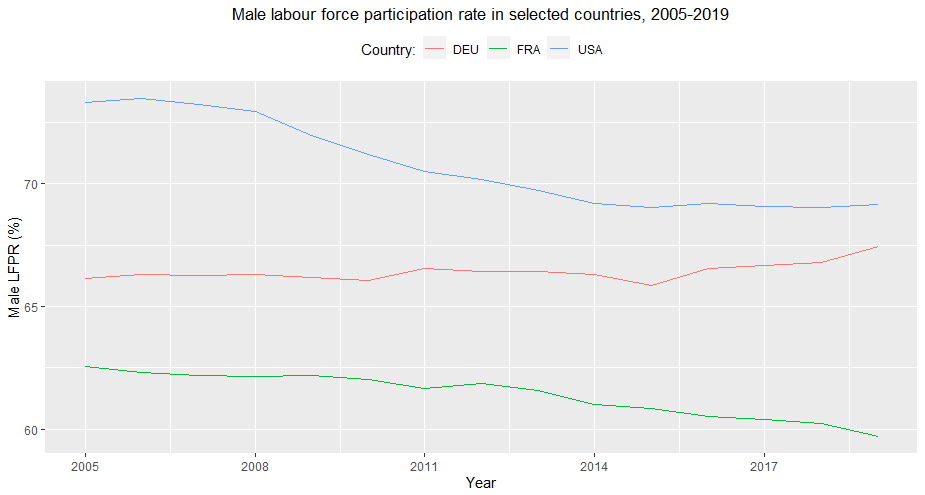

You can also build interesting (and visually telling) stacked columns or bars.

For example, based on ILOSTAT data, you can plot the distribution of employed persons by economic class (defined according to the household’s per capita income/consumption per day). You can even do it with several disaggregations: in the example below, we chose to show the employment distribution by economic class separately for men and women and for youth and adults. From this figure, we clearly understand that working poverty (being poor in spite of being employed) affects youth much more than adults, and women more than men.

require(Rilostat)
if(!require(ggplot2)){install.packages('ggplot2')}
if(!require(dplyr)){install.packages('dplyr')}

    get_ilostat(id = 'EMP_2EMP_SEX_AGE_CLA_DT_A', 
                filters = list( ref_area = 'ZAF', 
                                time = '1999', 
                                sex = c('M', 'F'), 
                                classif1 = c('Y15-24', 'YGE25'))) %>% 
    filter(!classif2 %in% 'CLA_ECOCLA_TOTAL') %>% 
    mutate( sex =       factor(sex) %>% recode_factor(
                                'SEX_M' = 'Male', 
                                'SEX_F' = 'Female'), 
            classif1 =  factor(classif1) %>% recode_factor(
                                'AGE_YTHADULT_YGE25' = 'Adult', 
                                'AGE_YTHADULT_Y15-24' = 'Youth'),
            classif2 =  factor(classif2) %>% recode_factor(
                                'CLA_ECOCLA_USDLT2' = '<US$1.9', 
                                'CLA_ECOCLA_USDGE2LT3' = '>=US$1.9 & <US$3.2', 
                                'CLA_ECOCLA_USDGE3LT5' = '>=US$3.2 & <US$5.5', 
                                'CLA_ECOCLA_USDGE5' = '>=US$5.5')) %>% 
    ggplot(aes(y=obs_value, x=as.factor(classif1), fill=classif2)) +
    geom_bar(stat="identity") +
    facet_wrap(~as.factor(sex)) + coord_flip() +
    theme(legend.position="top") +
    ggtitle("Employment by economic class, sex and age, South Africa, 1999") +
    labs(x="Age group", y="Distribution of economic class (%)", fill="Economic class : ") + 
    theme(plot.title = element_text(hjust = 0.5)) + 
    scale_fill_brewer(type = "div")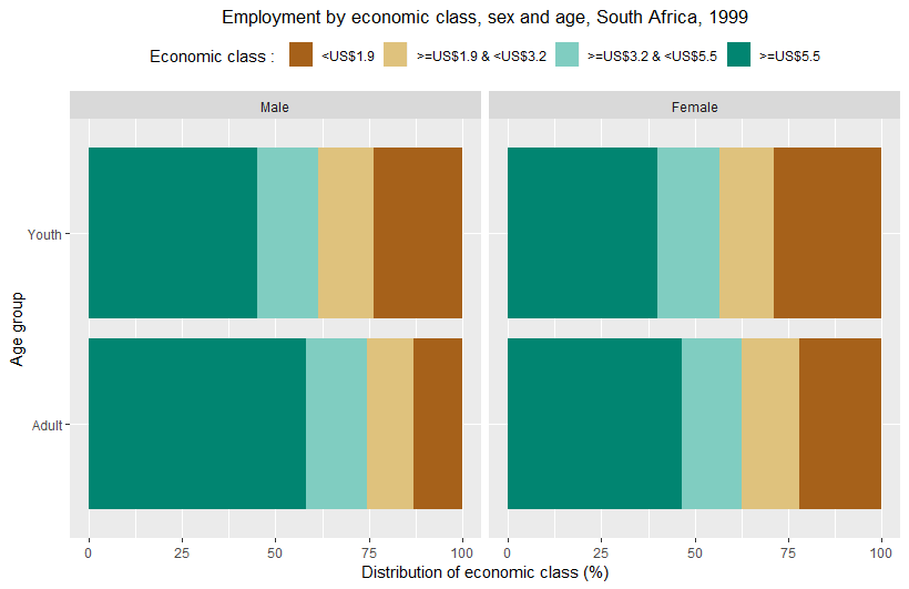

You can also combine the ilostat package with other packages to create triangular graphs, plotting three different indicators which relate to the same topic and whose observations are mutually exclusive.

You can use this type of graph, for instance, to visually convey the share of the employed population working in agriculture, industry and services, all three compared, and even more revealing, compare this across countries.

In the example below, we used three different indicators of labour underutilization (unemployment, time-related underemployment and discouraged job-seekers) to study how they are inter-related in selected countries. These three population groups are all mutually exclusive, but they are all part of the broad category of labour underutilization. Unemployment represents all persons not in employment, available for employment and actively seeking employment, while discouraged job-seekers are those persons not in employment and available for employment who do not actively look for employment for specific reasons having to do with the situation in the labour market, and time-related underemployment refers to persons in employment who would like to work more hours and are available to work more hours than their current working time. The graph below brings to light the differences across countries in the labour underutilization composition, by showing where unemployment is the biggest concern, as opposed to time-related underemployment or discouragement.

require(Rilostat)
if(!require(tidyr)){install.packages('tidyr')}
if(!require(dplyr)){install.packages('dplyr')}
if(!require(plotrix)){install.packages('plotrix')}
if(!require(stringr)){install.packages('stringr')}

triangle <- get_ilostat(id = c('EIP_WDIS_SEX_AGE_NB_A', 
                               'UNE_TUNE_SEX_AGE_NB_A', 
                               'TRU_TTRU_SEX_AGE_NB_A'), 
                        filters = list(
                                      ref_area = c('ZAF', 'MNG', 'CHL'), 
                                      source = 'BA',
                                      sex = 'SEX_T', 
                                      classif1 = 'YGE15', 
                                      time = '2013'),
                              detail = 'dataonly', 
                              cmd = "dat %>% select(ref_area, indicator, obs_value)", 
                              quiet = TRUE) %>%
            label_ilostat() %>%
            group_by(ref_area.label) %>%
            mutate(obs_value = obs_value / sum(obs_value)) %>% ungroup() %>%
            mutate(indicator.label = indicator.label %>% 
                                      str_replace(fixed(' by sex and age (thousands)'), '')) %>%
            spread(indicator.label, obs_value)

par(cex=0.75, mar=c(0,0,0,0))
positions <- plotrix::triax.plot(
                      as.matrix(triangle[, c(2,3,4)]),
                      show.grid = TRUE,
                      main = 'Selected labour underutilization indicators',
                      label.points= FALSE, point.labels = triangle$ref_area.label,
                      col.axis="gray50", col.grid="gray90",
                      pch = 19, cex.axis=1.2, cex.ticks=0.7, col="grey50")
                     
                     
ind <- which(triangle$ref_area.label %in%  triangle$ref_area.label)

df <- data.frame(positions$xypos, geo =  triangle$ref_area.label)

points(df$x[ind], df$y[ind], cex=2, col="red", pch=19)

text(df$x[ind], df$y[ind], df$geo[ind], adj = c(0.5,-1), cex=1.5)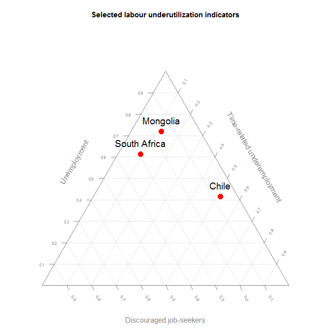

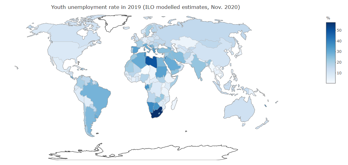
It is also possible to create maps showing how indicators behave across the world at a given point in time (static maps) or even through time (dynamic maps allowing the user to scroll over the available time period).

For instance, below we have built a map to see differences across the world in the youth unemployment rate. For this, we have selected data from a compilation which is methodologically robust and consistent across countries to ensure international comparability: the ILO modelled estimates (from November 2017). You can change the legend settings to use the color coding that best suits your data. In our case, the colour scale used allows us to quickly see that youth unemployment rates are particularly high in Southern and Northern Africa.

require(Rilostat)
if(!require(plotly)){install.packages('plotly')}
if(!require(dplyr)){install.packages('dplyr')}
if(!require(stringr)){install.packages('stringr')}

dat <- get_ilostat(id = 'UNE_2EAP_SEX_AGE_RT_A', filters = list(
                                time = '2019', 
                                sex = 'SEX_T', 
                                classif1 = 'AGE_YTHADULT_Y15-24'
                                )) %>% 
            filter(!str_sub(ref_area,1,1) %in% 'X') %>% 
            select(ref_area, obs_value) %>% 
            left_join(  Rilostat:::ilostat_ref_area_mapping %>% 
                            select(ref_area, ref_area_plotly)%>% 
                            label_ilostat(code = 'ref_area'), 
                        by = "ref_area") %>% 
            filter(!obs_value %in% NA)

    
            
dat %>% 
    plot_geo( 
            z = ~obs_value, 
            text = ~ref_area.label, 
            locations = ~ref_area_plotly
        ) %>% 
        add_trace(
            colors = 'Blues',
            marker = list(
                        line = list(
                            color = toRGB("grey"), 
                            width = 0.5)
                    ), 
            showscale = TRUE
        ) %>%
        colorbar(
            title = '%', 
            len = 0.5
        ) %>%
        layout(
          title = 'Youth unemployment rate in 2019 (ILO modelled estimates, Nov. 2020)', 
          geo = list(   
                    showframe = FALSE,  
                    showcoastlines = TRUE,
                    projection = list(type = 'natural earth'), 
                    showcountries = TRUE, 
                    resolution = 110) # or 50
            )

Contact information

For further information on the ilostat R package, please contact:

ILO Department of Statistics (ilostat@ilo.org)

For specific issues concerning code source, please report on github

For questions related to the ilostat database contact (ilostat@ilo.org) or visit ilostat website

Permission to reproduce ILO publication and data: the reproduction of ILO material is generally authorized for non-commercial purposes and within established limits. However, you may need to submit a formal request in certain circumstances. for more information please refer to:

Bulk download in ILOSTAT:

ILO Department of Statistics

2024-09-03